On January 16, I attended the CSCAR workshop on open source GIS basics presented by Manish Verma. As the Design Lab is working with biodiversity data for several projects, I figured that being exposed to some fundamentals about GIS could be useful since location metadata is a crucial aspect of biodiversity records.
What immediately struck me is that we didn’t start by pulling up a map, or even by opening the GIS software. The workshop began with the presenter emphatically reminding us that in order to understand any sort of digital data, you need to know what data model you are working with. Digital data is stored in a computer in some format, according to a particular set of standards, each of which bears information about what the data means, how it will be represented, and how you can manipulate it. For GIS data, he said that it is usually thought of as following one of three data models:
- Entity model, where locations and geographical features are treated as separate entities
- Field model, where a region is separated into many subregions on a grid pattern, each of which has information about what is present in that location (think pixels in a raster image)
- Network model, where geographic data is expressed via a system of nodes and edges (sort of like graphs in graph theory, except in the case of geographical data, distances matter)
These are merely rough restatements of the basic rundown - if you plan on working with GIS data extensively, you will want more rigorous definitions of these data models. The important thing to note here is that these are three different approaches to (digitally) capturing how locations exist relative to one another in the context of physical space.
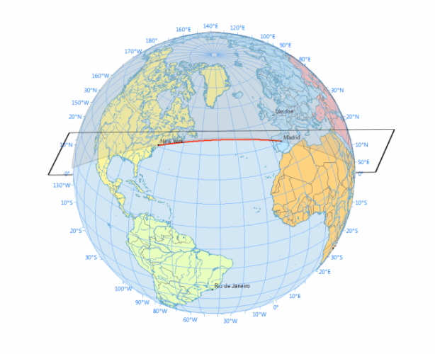
Next, we covered some basics of coordinate systems. One central point he emphasized here is that latitude and longitude should always be understood as a means to pinpoint a location on the surface of a spheroid. This is essentially the entire reason we use a pair of angles rather than simpler Euclidean geometry. Use of different models of Earth will result in slightly different implementations of latitude and longitude. He mentioned that a model called WSG84 is typically the standard. Switching from Lat/Long to 2D planar coordinates always requires projection, and there are many, many possible projections to choose from. The other central point he made during this section is that going from a 3D surface to a 2D plane always introduces geometrical (but, importantly, not topological) distortions in at least one of the following: shape, area, distance, and direction. Selecting a projection system involves asking which of those four characteristics matters the most for your particular application, then selecting a projection which best preserves the accuracy and geographic integrity of that characteristic. Here is a neat little video going over this point in a more visual way.
It is useful to keep in mind that we live on the surface of a sphere, not a 2D surface, for it matters a great deal when travelling large distances (hence, e.g., airline paths following great circle geodesics rather than “straight lines”).
https://gisgeography.com/great-circle-geodesic-line-shortest-flight-path/
A third point he made sure to emphasize here is that, due to the significant differences between a 3D model and projections, and between different projections, one must always be sure to convert data in different coordinate reference systems (CRSs) to the same CRS before comparing or combining it, or really before doing any sort of analysis.
Pivoting back to data models, he discussed how the world is represented in the entity data model. Every entity in the model can be represented with three “primitives” - points, lines, and polygons. More complex objects can be built by combining these primitives. A point is a set of two numbers - a single set of coordinates. A line is an ordered set of points, which are connected by straight line segments when displayed by the software. A polygon is a set of points where the first and last point are the same, creating a closed geometric shape. He called this the “Vector data model,” or just vector data. So, ultimately, in this model a geographic location or feature can be specified by four things (or sets of things) -
- the type of geometry it is (point, line, or polygon)
- the coordinates
- the CRS being used, and
- any additional descriptive attributes (e.g. name of place)
This model is the one used by the common Environmental Systems Research Institute (Esri) shapefile format, which was introduced along with their ArcView GIS software (the precursor to ArcGIS) and is a widely used file format for GIS data. A shapefile has three mandatory files (.shp, .shx, .dbf) and a host of optional files with a variety of other file extensions. The .shp file contains the feature geometry itself (points, lines, and polygons). Because the shapefile format is proprietary (as well as clunky and size-restricted), he mentioned that there is some interest in pushing for a more modern, open standard such as GeoJSON. However, it is important to understand shapefiles since so much current and legacy GIS data is in this format, and it will likely be around for a long time.
The main application we used during the workshop is an open source GIS application called QGIS. It would be difficult, and likely uninteresting, to try and walk through the same steps here as we did in the workshop. However, I can say that what I picked up is that creating various layers that contain the feature geometry (this layer has points, this layer has lines, and so on) is an important task in creating GIS data. Since different tasks are best served by different choices of CRS, knowing where to find these options, and knowing how to reproject datasets to match the CRS you’re currently using are important bits of information to have. We did some example tasks working with the local Ann Arbor region, so instead of using a Lat/Long CRS, we chose a 2D system known to be accurate for southeast Michigan (one of the State Plane projections). QGIS is able to read data from a variety of sources, such as spreadsheets and databases, as well as from raster images. Having worked with regular JSON before, I found GeoJSON to be a relatively easy format to understand and work with, so I hope it gains more traction in the field soon.
Another useful set of features of QGIS involves selecting features based on how they spatially interact with other features. The example we worked with in the workshop involved coordinates of crime events within the boundary of the city of Detroit. The framework he mentioned for conceptualizing these interactions is called DE-9IM, a topological model which defines categories of interaction such as “Equals”, “Disjoint”, “Intersects”, “Touches”, “Crosses”, “Within”, “Contains” and “Overlaps.” While most of these accords well with colloquial usage, they also have a specific mathematical meaning, hence the quotations.
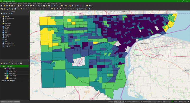
Lastly, we did a little work in R. R is a powerful, open source statistical language that is great for working with data like census data. We used R to download and tidy up some census data with median household income and geographical tracts for the city of Detroit. Using the simple features (sf) package, this data, once it is in the form you’d like, can be written out as shapefiles to be loaded into QGIS. The simple features package allows us to work with spatial vector data in R, meaning data that has the four features I mentioned above (CRS, coordinates, geometry type, and other attributes). Once we loaded this data into QGIS, we overlaid it onto a map of Detroit, then color coded tracts by median household income to get an “income map” of Detroit. He mentioned that this would allow us to make things like infographics with census data and other similar data.
That was a lot of information! My main takeaways from all of this are, location is always specific to a particular coordinate reference system. Different coordinate reference systems represent different models of Earth thus, data in different CRSs should be converted or reprojected to be in the same CRS before analysis. Spatial vector data is a collection of four sets of features that combine to tell us about geographical locations. And finally, that there are powerful open source tools for working with GIS that are just as functional as more popular proprietary applications like ArcGIS. If you will need to work with GIS data in the near future, I recommend looking into all of these things to get a grasp on them before diving in.